On Optimal, Minimal BRDF Sampling for Reflectance Acquisition
Nielsen, J. B.; Jensen, H. W.; Ramamoorthi R.
Introduction
This website contains supplementary code and data for the paper On Optimal, Minimal BRDF Sampling for Reflectance Acquisition to appear in Siggraph Asia 2015 Technical Papers.
Code covers python scripts for reconstructing BRDFs and determining optimum sampling directions, and the data includes our results for optimum sampling directions, precomputed principal components for your own reconstructions, and a small collection of reconstructed BRDFs in the MERL format.You are welcome to freely use any of the code and data provided on this website, but we kindly ask that you cite our paper. Please see citation.
Download supplementary material (pdf)
Code
Files
Python code has been made available for others to run their own optimizations and reconstructions. The code is arranged in a set of files:
- merlFunctions.py: Tools for reading the MERL BRDF files into python.
- coordinateFunctions.py: Various tools for converting coordinates (e.g. Rusinkiewicz to/from MERL, spherical coords, or direction vectors).
- optimizationFunctions.py: Functions for doing gradient descent optimization on condition number.
- reconstructionFunctions.py: Tools for reconstructing BRDFs.
In addition, example code is available for learning data statistics, optimizing sampling directions, and reconstructing data. The contents of these examples are shown below.
Download source files (Python)
Example: Training (exampleTraining.py)
In this example we simply load the MERL database, map it using our proposed "Log-Relative" mapping, and perform PCA. For performance, we precompute a mask map and a cosine map, used in other examples.
The MERL BRDF database can be downloaded here.
import numpy as np
import os.path as path
from os import listdir
from trainingFunctions import *
from merlFunctions import *
from coordinateFunctions import *

MERLDir = "MERLDir/"
OutputDir = "data/"

#Parse filenames
materials = [brdfFile for i,brdfFile in enumerate(listdir(MERLDir)) \
                if (path.isfile(MERLDir+brdfFile)
                and path.splitext(brdfFile)[1] == ".binary")]

#Fill observation array
obs = np.zeros((90*90*180, 3*len(materials)),'float32')
#Add each color channel as a single observation
for i in range(0,len(materials)):
    mat = readMERLBRDF("%s/%s"%(MERLDir,materials[i]))
    obs[:,3*i] = np.reshape(mat[:,:,:,0],(-1))
    obs[:,3*i+1] = np.reshape(mat[:,:,:,1],(-1))
    obs[:,3*i+2] = np.reshape(mat[:,:,:,2],(-1))

#Pre-compute maskMap (VERY SLOW if horizonCheck=True)
maskMap = ComputeMaskMap(obs, horizonCheck=False)

#Pre-compute cosine-map (VERY SLOW! - do once and store, or download!)
cosMap = ComputeCosMap(maskMap)

#Perform PCA on data
(scaledPCs,relativeOffset,median) = LearnMapping(obs,maskMap,cosMap)

#Save data
np.save('%s/MaskMap'%OutputDir,maskMap)
np.save('%s/CosineMap'%OutputDir,cosMap)
np.save('%s/ScaledEigenvectors'%OutputDir,scaledPCs)
np.save('%s/Median'%OutputDir,median)
np.save('%s/RelativeOffset'%OutputDir, relativeOffset)
Example: Optimization (exampleOptimization.py)
In this example we load the learned principal components etc. from training, and find the optimal up to 3 sampling directions
import numpy as np
from optimizationFunctions import *

#Load precomputed data
dataDir = "data/"
maskMap = np.load('%s/MaskMap.npy'%dataDir)   #Indicating valid regions in MERL BRDFs
Q = np.load('%s/ScaledEigenvectors.npy'%dataDir) #Scaled eigenvectors, learned from trainingdata

#Find up to 3 optimal sampling directions of Vs:
(pointHierachi, C) = FewToMany(Q, maskMap, 3)

#Print points: (in MERL coordinates)
for (i,pointSet) in enumerate(pointHierachi):
    print "#Optimum directions, n=%d:\n%s\n"%(i+1,pointSet)
Output from example:
#Optimum directions, n=1:
[[ 6  0 66]]

#Optimum directions, n=2:
[[  2  12  47]
 [158  37   4]]

#Optimum directions, n=3:
[[ 11  12   3]
 [154  69  15]
 [143  28  78]]
Example: Reconstruction (exampleReconstruction.py)
Here we have 5 RGB BRDF observations captured from 5 unique directions. Using the training data we reconstruct the full BRDF and store it in the MERL format
import numpy as np
from merlFunctions import *
from coordinateFunctions import *
from reconstructionFunctions import *

#BRDF observations (5 RGB values)
obs = np.array([[0.09394814, 0.01236500, 0.00221087],
                [0.09005638, 0.00315711, 0.00270478],
                [1.38033974, 1.21132099, 1.19253075],
                [0.97795460, 0.85147798, 0.84648135],
                [0.10845871, 0.05911538, 0.05381590]])

#Coordinates for observations (phi_d, theta_h, theta_d)
coords = np.array([[36.2,  1.4,  4.0 ],
                   [86.5,  76.7, 13.1],
                   [85.5,  7.6,  78.9],
                   [144.8, 2.5,  73.8],
                   [80.4,  12.9, 51.6]])

#Convert to BRDF coordinates
MERLCoords = RusinkToMERL(np.deg2rad(coords))
#Convert to IDs (i.e. rows-ids in the PC matrix)
MERLIds = MERLToID(MERLCoords)

#Load precomputed data
dataDir = "data/"
maskMap = np.load('%s/MaskMap.npy'%dataDir)   #Indicating valid regions in MERL BRDFs
median = np.load('%s/Median.npy'%dataDir)     #Median, learned from trainingdata
cosMap = np.load('%s/CosineMap.npy'%dataDir)  #Precomputed cosine-term for all BRDF locations (ids)
relativeOffset = np.load('%s/RelativeOffset.npy'%dataDir) #Offset, learned from trainingdata
Q = np.load('%s/ScaledEigenvectors.npy'%dataDir) #Scaled eigenvectors, learned from trainingdata

#Reconstruct BRDF
recon = ReconstructBRDF(obs, MERLIds, maskMap, Q, median, relativeOffset, cosMap, eta=40)
#Save reconstruction as MERL .binary
saveMERLBRDF("reconstruction.binary",recon)
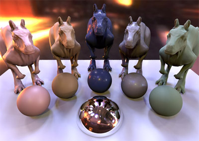
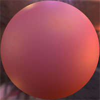
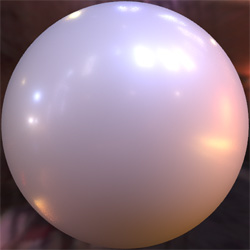
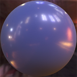
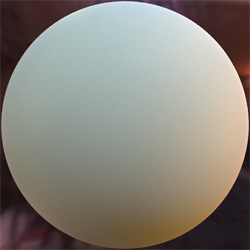
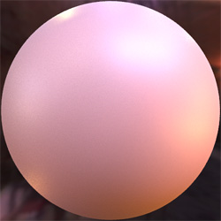
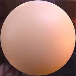
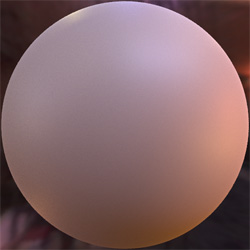
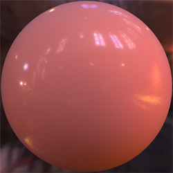
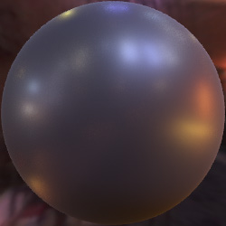
Rendering of reconstructed BRDF. (Note that code for rendering is not available here. See PBRT.)
Data
Direction files
Direction-lists are stored in the Numpy text format (.nptxt). To load the lists into python, simply do:
import numpy as np
directions = np.loadtxt("path/to/file.nptxt")
Directions are stored in n x 3 arrays, with n being the number of directions and the columns representing the 3 Rusinkiewicz coordinates in degrees (PhiD, ThetaH, ThetaD):
# phiD thetaH thetaD [deg]
24.13 01.63 40.45
52.29 29.02 21.24
Below direction lists can be downloaded for two different BRDF sampling approaches:
- Point sampling: A classical gonioreflectometer setup where a single point on the sample is illumnated from a point light source placed in one direction, and observed by a radiometer from a second direction
- Sphere sampling: A spherical, isotropic, sample is illuminated by a point light source placed in one direction, and observed by a camera from a second direction.
Precomputed data
We here supply precomputed data for users who are not interrested in acquiring the MERL database and performning principal component analysis etc. themselves.
The data is packed in a rar-container and includes:
- MaskMap: Refined list of valid indices where MERL BRDF values are valid.
- CosineMap: Cosine weights corresponding to the valid MERL BRDF values.
- ScaledEigenvectors: Principal Components of valid parts of mapped MERL BRDFs (i.e. the matrix Q).
- Median: Median of valid parts of MERL BRDFs (this is the reference BRDF for mapping, rho_ref).
- RelativeOffset: The mean of the mapped MERL BRDFs (used to zero-center data before PCA, mu_hat).
Download precomputed data (Python)
Reconstructed BRDFs
The following files are reconstructed BRDFs. The reconstructions are stored in the MERL BRDF format (.binary, see MERL Database).
Green cloth
Diffuse green cloth with some retroreflectivity. Reconstructed from 20 samples.
Miscallaneous
Citation
If you use the code or measurements, please, reference the following paper:
BibTeX:

@article {Nielsen2015,
	author = {Jannik Boll Nielsen and Henrik Wann Jensen and Ravi Ramamoorthi},
	title = {On Optimal, Minimal BRDF Sampling for Reflectance Acquisition},
	journal = {ACM Transactions on Graphics (TOG)},
	year = {2015},
	month = {November},
	volume = {34},
	number = {6},
	pages = {186:1-186:11},
	doi = {10.1145/2816795.2818085}
}